Mathematical Geoenergy

Our book Mathematical Geoenergy presents a number of novel approaches that each deserve a research paper on their own. Here is the list, ordered roughly by importance (IMHO):

1. Laplace’s Tidal Equation Analytic Solution.
   (Ch 11, 12) A solution of a Navier-Stokes variant along the equator. Laplace’s Tidal Equations are a simplified version of Navier-Stokes and the equatorial topology allows an exact closed-form analytic solution. This could classify for the Clay Institute Millenium Prize if the practical implications are considered, but it’s a lower-dimensional solution than a complete 3-D Navier-Stokes formulation requires.
2. Model of El Nino/Southern Oscillation (ENSO).
   (Ch 12) A tidally forced model of the equatorial Pacific’s thermocline sloshing (the ENSO dipole) which assumes a strong annual interaction. Not surprisingly this uses the Laplace’s Tidal Equation solution described above, otherwise the tidal pattern connection would have been discovered long ago.
3. Model of Quasi-Biennial Oscillation (QBO).
   (Ch 11) A model of the equatorial stratospheric winds which cycle by reversing direction ~28 months. This incorporates the idea of amplified cycling of the sun and moon nodal declination pattern on the atmosphere’s tidal response.
4. Origin of the Chandler Wobble.
   (Ch 13) An explanation for the ~433 day cycle of the Earth’s Chandler wobble. Finding this is a fairly obvious consequence of modeling the QBO.
5. The Oil Shock Model.
   (Ch 5) A data flow model of oil extraction and production which allows for perturbations. We are seeing this in action with the recession caused by oil supply perturbations due to the Corona Virus pandemic.
6. The Dispersive Discovery Model.
   (Ch 4) A probabilistic model of resource discovery which accounts for technological advancement and a finite search volume.
7. Ornstein-Uhlenbeck Diffusion Model
   (Ch 6) Applying Ornstein-Uhlenbeck diffusion to describe the decline and asymptotic limiting flow from volumes such as occur in fracked shale oil reservoirs.
8. The Reservoir Size Dispersive Aggregation Model.
   (Ch 4) A first-principles model that explains and describes the size distribution of oil reservoirs and fields around the world.
9. Origin of Tropical Instability Waves (TIW).
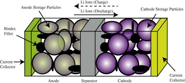
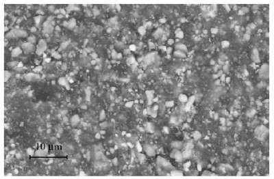
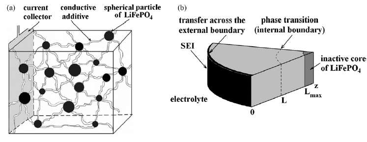
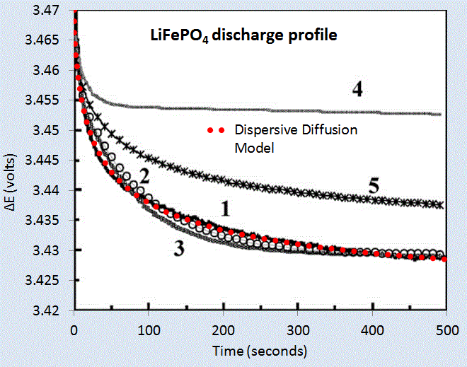
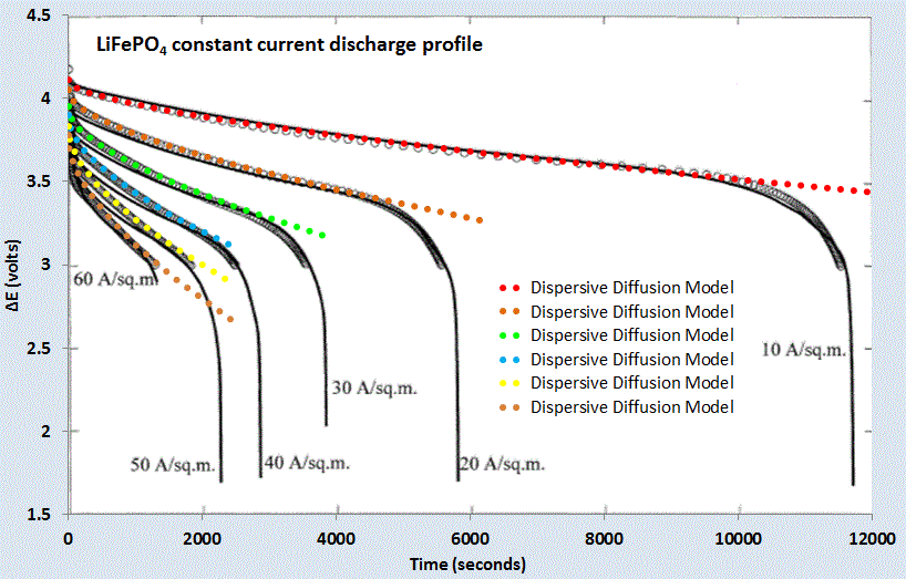
   (Ch 12) As the ENSO model was developed, a higher harmonic component was found which matches TIW
10. Characterization of Battery Charging and Discharging.
    (Ch 18) Simplified expressions for modeling Li-ion battery charging and discharging profiles by applying dispersion on the diffusion equation, which reflects the disorder within the ion matrix.
11. Anomalous Behavior in Dispersive Transport explained.
    (Ch 18) Photovoltaic (PV) material made from disordered and amorphous semiconductor material shows poor photoresponse characteristics. Solution to simple entropic dispersion relations or the more general Fokker-Planck leads to good agreement with the data over orders of magnitude in current and response times.
12. Framework for understanding Breakthrough Curves and Solute Transport in Porous Materials.
    (Ch 20) The same disordered Fokker-Planck construction explains the dispersive transport of solute in groundwater or liquids flowing in porous materials.
13. Wind Energy Analysis.
    (Ch 11) Universality of wind energy probability distribution by applying maximum entropy to the mean energy observed. Data from Canada and Germany. Found a universal BesselK distribution which improves on the conventional Rayleigh distribution.
14. Terrain Slope Distribution Analysis.
    (Ch 16) Explanation and derivation of the topographic slope distribution across the USA. This uses mean energy and maximum entropy principle.
15. Thermal Entropic Dispersion Analysis.
    (Ch 14) Solving the Fokker-Planck equation or Fourier’s Law for thermal diffusion in a disordered environment. A subtle effect but the result is a simplified expression not involving complex errf transcendental functions. Useful in ocean heat content (OHC) studies.
16. The Maximum Entropy Principle and the Entropic Dispersion Framework.
    (Ch 10) The generalized math framework applied to many models of disorder, natural or man-made. Explains the origin of the entroplet.
17. Solving the Reserve Growth “enigma”.
    (Ch 6) An application of dispersive discovery on a localized level which models the hyperbolic reserve growth characteristics observed.
18. Shocklets.
    (Ch 7) A kernel approach to characterizing production from individual oil fields.
19. Reserve Growth, Creaming Curve, and Size Distribution Linearization.
    (Ch 6) An obvious linearization of this family of curves, related to Hubbert Linearization but more useful since it stems from first principles.
20. The Hubbert Peak Logistic Curve explained.
    (Ch 7) The Logistic curve is trivially explained by dispersive discovery with exponential technology advancement.
21. Laplace Transform Analysis of Dispersive Discovery.
    (Ch 7) Dispersion curves are solved by looking up the Laplace transform of the spatial uncertainty profile.
22. Gompertz Decline Model.
    (Ch 7) Exponentially increasing extraction rates lead to steep production decline.
23. The Dynamics of Atmospheric CO2 buildup and Extrapolation.
    (Ch 9) Convolving a fat-tailed CO2 residence time impulse response function with a fossil-fuel emissions stimulus. This shows the long latency of CO2 buildup very straightforwardly.
24. Reliability Analysis and Understanding the “Bathtub Curve”.
    (Ch 19) Using a dispersion in failure rates to generate the characteristic bathtub curves of failure occurrences in parts and components.
25. The Overshoot Point (TOP) and the Oil Production Plateau.
    (Ch 8) How increases in extraction rate can maintain production levels.
26. Lake Size Distribution.
    (Ch 15) Analogous to explaining reservoir size distribution, uses similar arguments to derive the distribution of freshwater lake sizes. This provides a good feel for how often super-giant reservoirs and Great Lakes occur (by comparison).
27. The Quandary of Infinite Reserves due to Fat-Tail Statistics.
    (Ch 9) Demonstrated that even infinite reserves can lead to limited resource production in the face of maximum extraction constraints.
28. Oil Recovery Factor Model.
    (Ch 6) A model of oil recovery which takes into account reservoir size.
29. Network Transit Time Statistics.
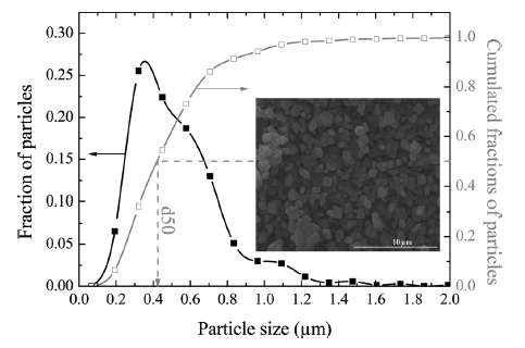
    (Ch 21) Dispersion in TCP/IP transport rates leads to the measured fat-tails in round-trip time statistics on loaded networks.
30. Particle and Crystal Growth Statistics.
    (Ch 20) Detailed model of ice crystal size distribution in high-altitude cirrus clouds.
31. Rainfall Amount Dispersion.
    (Ch 15) Explanation of rainfall variation based on dispersion in rate of cloud build-up along with dispersion in critical size.
32. Earthquake Magnitude Distribution.
    (Ch 13) Distribution of earthquake magnitudes based on dispersion of energy buildup and critical threshold.
33. IceBox Earth Setpoint Calculation.
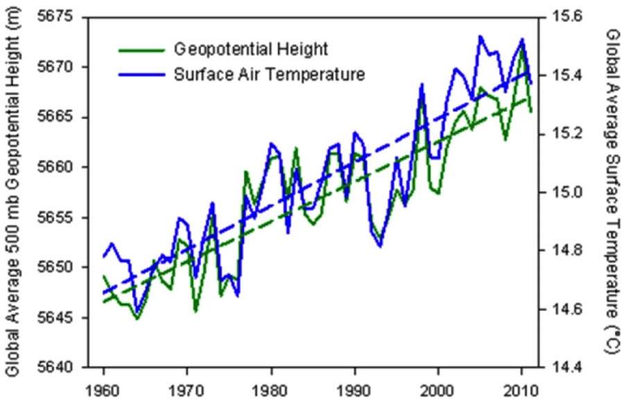
    (Ch 17) Simple model for determining the earth’s setpoint temperature extremes — current and low-CO2 icebox earth.
34. Global Temperature Multiple Linear Regression Model
    (Ch 17) The global surface temperature records show variability that is largely due to the GHG rise along with fluctuating changes due to ocean dipoles such as ENSO (via the SOI measure and also AAM) and sporadic volcanic eruptions impacting the atmospheric aerosol concentrations.
35. GPS Acquisition Time Analysis.
    (Ch 21) Engineering analysis of GPS cold-start acquisition times. Using Maximum Entropy in EMI clutter statistics.
36. 1/f Noise Model
    (Ch 21) Deriving a random noise spectrum from maximum entropy statistics.
37. Stochastic Aquatic Waves
    (Ch 12) Maximum Entropy Analysis of wave height distribution of surface gravity waves.
38. The Stochastic Model of Popcorn Popping.
    (Appx C) The novel explanation of why popcorn popping follows the same bell-shaped curve of the Hubbert Peak in oil production. Can use this to model epidemics, etc.
39. Dispersion Analysis of Human Transportation Statistics.
    (Appx C) Alternate take on the empirical distribution of travel times between geographical points. This uses a maximum entropy approximation to the mean speed and mean distance across all the data points.

Rating of Climate Change blogs

Scientific blogging is on a decline and that is especially evident with respect to climate change blogs. Nothing really good left apart from forums such as https://forum.azimuthproject.org/discussions (which allows equation markup, image posting, and freedom to create threaded discussions).

Here is a grading of blogs that I have on my RSS feed:

• WUWT :  F-
  A horrible AGW denier blog that pretends to be fair & balanced. RSS feed does not work with Owl.
• Tallbloke's Talkshop : F-
  A horrible AGW denier blog that specializes in numerology
• Real Climate : C
  Sparse postings and comment moderation has long latencies so the discussion is glacially paced
• Open Mind : C
  Not very interesting, mostly from a statistical angle, which is not where progress in analysis occurs
• Science of Doom : D
  I don't understand this site, seems to be run by a thinly veiled skeptic. Might as well read books by Pierrehumbert to gain an understanding of the physics instead of struggling along with the topics.
• And Then There's Physics : D+
  The moderators are control freaks, and the discussions are safe as milk
• Peak Oil Barrel : A
  A very good blog that allows both fossil fuel discussion and climate change discussion, separated in distinct threads.  Moderated slightly and images allowed, along with short-term editing.
• The Blackboard : F-
  An awful blog run by a mechanical engineer which at one point had climate science discussion but now consists of pro-Trump cheerleading.
• Clive Best : D+
  The moderator tries hard but then stumbles as he desperately tries to debunk the AGW consensus. Marginally better than Science of Doom because at least the scientific ideas are creative.
• Climate Audit : F-
  Awful conspiracy-laden blog run by a former Canadian mining executive.
• Climate Etc : F-
  Pointless blog stressing climate science uncertainty run by a now-retired climate science professor J. Curry with a comment section that seems infested with Australian AGW deniers. 
• Moyhu : B
  Halfway-decent posts by a retired fluid dynamics researcher but an ugly and unstable comment-entry system. 
• Hotwhopper : C+
  Well-thought out counter-attacks to nonsense at sites such as WUWT, but nothing really about discussions of science
• Robert Scribbler : C
  The American version of HotWhopper, with probably too much doom & gloom.
• Skeptical Science: D
  Nothing interesting here as they never seem to veer from the consensus.  The comments seem to be overly moderated and at one time the RSS feed was broken, but that has recently been fixed.
• Roy Spencer, PhD : F-
  Horrible blog by a religious zealot with comments infested by AGW deniers
• Rabbet Run : B-
  Below Moyhu because nothing really innovative but occasional insight
• More Grumbine Science : B
  By a NASA guy,  posts very rarely

This is a previous summary I had written two years ago (I had forgotten I had saved it in a draft folder, and so you can see how little has changed)

Blog	Grade	Rationale
Real Climate	C	Too long turnaround for comments
And Then There's Physics	D	Too much ClimateBall
Skeptical Science	D	Too insular, won't discuss cutting edge
Science of Doom	D-	Inflitrated by deniers
Open Mind	C	Too much on statistics, which does a disservice to unlocking deterministic aspects such as ENSO
Moyhu	B	Worst comment entry, but the research is quality
This Week in Science: DailyKos	C+	Nothing in depth
Watt's Up With That	F	Garbage
Tallbloke's Talkshop	F	Loony bin
The Blackboard	F	Nasty people
Climate Etc	F	Clueless (mainly Aussies) lead by a clueless
Roy Spencer	F	Zero real science
Rabbet Run	C	Too much inside posturing
Hot Whopper	C	Good if you want to see deniers get debunked
Robert Scribbler	C	Verges on hysterical but who knows
Azimuth Project	A	A true forum. Allows everyone to create markup and add charts

Context/Earth

Please refer to my new Wordpress blog Context/Earth for future posts.

Wordpress has better commenting options such as provisions for pictures and charts.

The scope of the blog is also more comprehensive, as it will include all environmental and energy topics tied together in a semantic web framework. 

Onward and upward as they say.

Expansion of atmosphere and ocean

This is a short tutorial together with some observational evidence explaining how the atmosphere and ocean is expanding measurably in the face of global warming.

Ocean thermal expansion

The ocean absorbs heat per area according to its heat capacity

$$ \Delta E = C_p \cdot \Delta T \cdot {Depth}$$

The linear coefficient of thermal expansion is assumed constant over a temperature range. Multiplying this over a depth:

$$ \Delta Z = \epsilon \cdot \Delta T \cdot Depth $$
But now we can substitute the total energy gained from the first equation:
$$ \Delta Z = \epsilon \frac{\Delta E}{C_p} $$
Assume that the linear coefficient of thermal expansion is 0.000207 per °C, and specific heat capacity is 4,000,000 J/m^3/°C.

If an excess forcing of 0.6 W/m^2 occurs over one year (see the OHC model), then the increase in the level of the ocean is

0.000207  * 0.6*(365*24*60*60) / 4,000,000 = 0.98 mm

This is called the steric sea-level rise, and it is just one component of the sea-level rise over time (the others have to do with melting ice). From the figure below, one can see that the thermal rise is close to 1mm/year over the last decade.

The red line shows the thermal expansion from the ocean heating. Thermal rise is 1 mm/year over the 3 mm/year total sea-level rise.

Atmosphere thermal expansion

The trick here is to infer the atmosphere expansion by looking at an equal pressure point as a function of altitude (a geopotential height isobar) and determine how much that point has increased over time.  I was able to find one piece of data from The Weather Channel's senior meteorologist Stu Ostro.

The geopotential height anomaly is shown below for the 500 mb (1/2 atmosphere)

Geopotential height anomaly @ 500 mb plotted alongside global temperature anomaly.

In absolute terms it is charted as follows:

Global average geopotential height @ 500 mb plotted alongside global temperature.
http://icons-ak.wxug.com/graphics/earthweek/geopotential-height-and-air-temperature.png

To understand how the altitude has changed, consider the classical barometric formula:
$$ P(H) = P_0 e^{-mgH/RT} $$

We take the point at which we reached 1/2 the STP of 1 atmosphere at sea-level:

$$ P(H)/P_0 = 0.5 = e^{-mgH/RT} $$

or
$$ H = RT/mg \cdot ln(2) $$
Assuming the average molecular weight of the atmospheric gas constituents does not change, the change in altitude (H) should be related to the change in temperature (T) by:
$$ \Delta H = R \Delta T / mg \cdot ln(2) $$
or
$$ \frac{ \Delta H}{\Delta T} =  \frac{R}{mg} ln(2) $$
For R = 8314, m=29, and g=9.8, the slope should be 29.25 *ln(2) = 20.3 m/°C.

From the linear regression agreement between the two, we get a value of 25.7 m/°C.

Linear regression between the geopotential height change and temperature change

Why is this geopotential height change about 26% higher than it should be from the theoretical value considering that the height should track the temperature according to the barometric formula?

If we use the polytropic approximation (equation 1 in the barometric formula), the altitudinal difference between the low temperature and high temperature 500 mb pressure values remains the same as when we use the classic exponential damped barometric formula:

If we apply the polytropic barometric formula instead of the exponential, we still show a real height change that is higher than theoretically predicted by ~25% at the 500 mb isobar.

This discrepancy could be due to measurement error, as the readings are taken by weather balloons and the accuracy could have drifted over the years.

It is also possible that the composition of the atmosphere could have changed slightly at altitude. What happens if the moisture increased slightly? This shouldn't make much difference.

Most likely is the possibility that the baseline sea-level pressure has changed, which shifted the 500 mbar point artificially. See http://www.ipcc.ch/publications_and_data/ar4/wg1/en/ch10s10-3-2-4.html.

"10.3.2.4 Sea Level Pressure and Atmospheric Circulation

As a basic component of the mean atmospheric circulations and weather patterns, projections of the mean sea level pressure for the medium scenario A1B are considered. Seasonal mean changes for DJF and JJA are shown in Figure 10.9 (matching results in Wang and Swail, 2006b). Sea level pressure differences show decreases at high latitudes in both seasons in both hemispheres. The compensating increases are predominantly over the mid-latitude and subtropical ocean regions, extending across South America, Australia and southern Asia in JJA, and the Mediterranean in DJF. Many of these increases are consistent across the models. This pattern of change, discussed further in Section 10.3.5.3, has been linked to an expansion of the Hadley Circulation and a poleward shift of the mid-latitude storm tracks (Yin, 2005). This helps explain, in part, the increases in precipitation at high latitudes and decreases in the subtropics and parts of the mid-latitudes. Further analysis of the regional details of these changes is given in Chapter 11. The pattern of pressure change implies increased westerly flows across the western parts of the continents. These contribute to increases in mean precipitation (Figure 10.9) and increased precipitation intensity (Meehl et al., 2005a). "

I will have to figure out the mean sea-level pressure change over this time period to verify this hypothesis.

The following recent research article looks into the shifts in geopotential height over shorter time durations:

[1]

Y. Y. Hafez and M. Almazroui, “The Role Played by Blocking Systems over Europe in Abnormal Weather over Kingdom of Saudi Arabia in Summer 2010,” Advances in Meteorology, vol. 2013, p. 20, 2013.

 

                   ADDED  7/8/2013                

One possibility for the larger-than-expected altitude change is that the average lapse rate has changed slightly.  We can use the lapse rate variation of the barometric formula, and perturb the lapse rate, L, around its average value:

$$ P(H) = P(0) (1- \frac{LH}{T_0})^{\frac{gm}{LR}} $$

Granted, the error bars on this calculation are significant but we can see how subtle the effect is.

Sea-level pressure, P(0) = 1013.25 mb
Gas constant,  R = 8.31446 J/K/mol
Earth's gravity, g = 9.807 m/s^2
Avg molecular weight, m = 0.02896 kg/m

In 1960, the temperature was about 14.65°C and 500 mb altitude was 5647 m.
In 2010, the temperature was about 15.4°C and 500 mb altitude was 5667 m.

All we need to do is invert the P(H) formula for each pair of values, modifying L slightly.

If we select a lapse rate, L, for 1960 of 0.0051°C/m, we calculate H = 5647.9m for P(H)=500 mb.
If we select a lapse rate, L, for 2010 of 0.0050°C/m, we calculate H = 5668.4m for P(H)=500 mb.

The difference in the two altitudes for a change in L of -0.0001°C/m is 20.5m, about what the geopotential height chart shows.

If we leave the L at 0.0051°C/m for both 1960 and 2010, the difference of the 500mb altitudes is only 14.7m.

To the extent that we can trust the numbers on the charts from Ostro, the change in geopotential height is suggesting a feedback effect in the lapse rate due to global warming.  The lapse rate is decreasing over time, which implies that the heat capacity of the atmosphere is increasing (likely due to higher specific humidity), thereby buffering changes in temperature with altitude.

This means that a given temperature increase at a particular altitude (where the CO2 IR window can achieve a radiative balance) will be reflected as a scale-modified temperature at sea level

In 1960, the temperature difference at 500mb altitude is 0.0051°C/m * 5647.9m = 28.80°C
In 2010, the temperature difference at 500mb altitude is 0.0050°C/m * 5668.4m = 28.34°C

The difference at sea-level from the chart is 15.4°C-14.65°C = 0.75°C whereas the difference at the 500mb altitude assuming the modified lapse rate is 0.75°C - 0.46°C = 0.29°C.  If the lapse rate didn't change then this sea-level difference would maintain at a constant atmospheric pressure isobar in altitude.

For implications in the interpretation, see page 24 of National Research Council Panel on Climate Change Feedbacks (2003). Understanding climate change feedbacks : National Academies Press. ISBN 978-0-309-09072-8.  They caution that the measurements require some precision, otherwise the errors can multiply due to the differences between two large numbers.

Characterization of Battery Charging and Discharging

I had the good fortune of taking a week long Society of Automotive Engineers (SAE) Academy class on hybrid/electric vehicles. The take-home message behind HEV and EV technology is to remember that a quality battery plus optimizing the management of battery cycling remain the keys to success.   That is not surprising --  we all know that gasoline has long been "king", and since current battery technology has nowhere near the energy density of gasoline, the battery has turned into a "diva".  In other words, it will perform as long as it is in charge (so to speak) and the battery is well maintained.

I can report that much class time was devoted to the electrochemistry of Lithium-ion batteries. Lithium is an ideal elemental material due to its position in the upper left-hand corner of the periodic table -- in other words a very lightweight material with a potentially high energy density.

What was surprising to me was the sparseness of detailed characterization of the material properties. One instructor stated that the lack of measured diffusion properties for battery cell specifications was a pet peeve of his.  Having these properties at hand allows a design engineer to better model the charging and discharging characteristics of the battery, and thus to perhaps to develop better battery management schemes. Coming from the semiconductor world, it is almost unheard of to do design without adequate device characteristics such as mobility and diffusivity.

From my perspective, this is not necessarily bad. Any time I see an anomalous behavior or missing piece, it opens the possibility I can fill a modeling niche.

Introduction

Modern rechargeable battery technology still relies on the principles of electro-chemistry and a reversible process, which hasn’t changed in fundamental terms since the first lead-acid battery came to market in the early 1900’s. What has changed is the combination of materials that make a low-cost, lightweight, and energy-efficient battery which will serve the needs of demanding applications such as electric and hybrid-electric vehicles (EV/HEV).

As energy efficient operation is dependent on the properties of the materials being combined, it is well understood that characterizing the materials is important to advancing the state-of-the-art (and in increasing EV acceptance).

Of vital importance is the characterization of diffusion in the electrode materials, as that is the rate-limiting factor in determining the absolute charging and discharging speed of the material-specific battery technology. Unfortunately, because of the competitive nature of battery producers, many of the characteristics are well-guarded and treated as trade secrets. For example, it is very rare to find diffusion coefficient characteristics on commercial battery specification sheets, even though this kind of information is vital for optimizing battery management schemes [7].

In comparison to the relatively simple diffusional mechanisms of silicon oxide growth, the engineered structure of well-designed battery cell presents a significant constraint to the diffusional behavior. In Figure 1 below we show a schematic of a single lithium-ion cell and the storage particles that charge and discharge. The disordered nature of the storage particles in Figure 2 is often described by what is referred to as a tortuosity measure.

Figure 1: Exaggerated three-dimensional view of a lithium-ion battery cell and the direction of current flow during charging and discharging

Figure 2 : Realistic view of the heavily disordered nature of the LiFePO4 storage particles [1].

The constraints on the diffusion is that it is limited in scale to that of the radius of the storage particle. The length scale is limited essentially to the values L to Lmax shown in Figure 3 below.

Figure 3 : Diffusion of ions takes place through the radial shell of the LiFePO4 spherical particle [1]. During the discharge phase, the ions need to migrate outward through shell and through the SEI barrier before reaching the electrolyte. At this point they can contribute to current flow.

The size of the particles also varies as shown in Figure 4 below.  The two Lithium-ion materials under consideration, LiFePO4 and LiFeSO4F, have different materials properties but are structurally very similar (matrixed particles of mixed size) so that we can use a common analysis approach.  This essentially allows us to apply uncertainty in the diffusion coefficient and uncertainties in the particle size to establish a common diffusional behavior formulation.

Figure 4 : Particle size distribution of FeSO4F spherical granules [2]. The variation in lengths and material diffusivities opens the possibility of applying uncertainty quantification to a model of diffusive growth.

Dispersive Diffusion Analysis of Discharging

The diffusion of ions through the volume of a spherical particle does have similarity to classical regimes such as the diffusion of silicon through silicon dioxide.  That process in fact leads to the familiar Fick's law of diffusion, whereby the growing layer of oxide follows a parabolic growth law (in fact this is a square root with time, but was named parabolic by the semiconductor technology industry for historical reasons, see for example here).

The model that we can use for Li+ diffusion derives from the classic solution to the Fokker-Planck equation of continuity (neglecting any field driven drift).
$$ \frac{\partial C}{\partial t} - D \nabla^2 C=0 $$ where C is a concentration and D is the diffusion coefficient.  Ignoring the spherical orientation, we can just assume a solution along a one dimensional radially outward axis, x:

$$ \large C(t,x|D) = \frac{1}{\sqrt{4 \pi D t}} e^{-x^2/{4 D t}} $$
This is a marginal probability which depends on the diffusion coefficient. Since we do not know the variance of the diffusivity, we can apply a maximum entropy distribution across D.
$$ \large p_d(D) = \frac{1}{D_0} e^{-D/D_0} $$
This simplifies the representation to the following workable formulation.
$$ \large C(t,x) = \frac{1}{2 \sqrt{D_0 t}} e^{-x/{\sqrt{D_0 t}}} $$
We now have what is called a kernel solution (i.e. Green's function) that we can apply to specific sets of initial conditions and forcing functions, the latter solved via convolution.

Fully Charged Initial Conditions
Assume the spherical particle is uniformly distributed with a charge density C(0, x) at time t=0.

Discharging Model
For every point along the dimensions of the particle of size L, we calculate the time it takes to diffuse to the outer edge, where it can enter the electrolytic medium.  This is simply an integral of the C(t, x) term for all points starting from x' = d to L, where d is the inner core radius.
$$  \large C(t) = \int_{d}^L C(t,L-x) dx $$
this integrates straightforwardly to this concise representation:
$$ \large C(t) = C_0 \frac{ 1 - e^{-(L-d)/{\sqrt{D_0 t}}} } {L - d} $$
The voltage of the cell is essentially the amount of charge available, so as this charge depletes, the voltage decreases in proportion.

We can test the model on two data sets corresponding to a LiPO4 cell [1] and a LiSO4F cell [2]. Figure 5 below shows the model fit for LiPO4 as the red dotted line, and which should be level-compared to the solid black line labelled 1. The other curves labelled 2,3,4,5 are alternative diffusional model approximations applied by Churikov et al that clearly do not work as well as the dispersive diffusion formulation derived above.
 

Figure 5 : Discharge profile of LiFePO4 battery cell [1], with the red dotted line showing the parameterized dispersive diffusion model.  The curves labelled 1 through 5 show alternative models that the authors applied to fit the data. Only the dispersive diffusion model duplicates the fast drop-off and long-time scale decline.

Figure 6 below shows the fit to voltage characteristics of a LiSO4F cell, drawn as a red dotted line above the light gray data points. In this case the diffusional model by Delacourt shown in solid black is well outside acceptable agreement.

Figure 6 : Discharge profile of LiFeSO4F battery cell [2], with the red dotted line showing the parameterized dispersive diffusion model.  The black curve shows the model that the authors applied to fit the data. 

The question is why does this simple formulation work so well? As with many similar cases of characterizing disordered material, the fundamentally derived solution needs to be adjusted to take into account the uncertainty in the parameter space.  However, this step is not routinely performed and by adding modeling details (see [4]) to try to make up for a poor fit works only as a cosmetic heuristic.   In contrast, by performing the uncertainty quantification, like we did with the diffusion coefficient, the first-order solution works surprisingly well with no need for additional detail.

Constant Current Discharge
Instead of assuming that the particle size is L, we can say that the L is an average and apply the same maximum entropy spread in values.
$$  \large C(t) = \int_{0}^{\infty} C(t,x) \frac{1}{L} e^{-x/L} dx $$
this integrates straightforwardly to this concise representation:
$$ \large C(t) = C_0 \frac{1}{ L + {\sqrt{D_0 t}} } $$
The reason we do this is to allow us to recursively define the change in charge to a current. In  this case, to get current we need to differentiate the charge with respect to time.
$$ \large I(t) = \frac{dC(t)}{dt}  $$
This differentiates to the following expression
$$ \large I(t) = - \frac{C_0}{ (L + {\sqrt{D_0 t}})^2} \frac{1}{2 \sqrt{t}} $$
But note that we can insert C(t) back in to the expression
$$ \large I(t) = \frac{C(t)}{(L + {\sqrt{D_0 t}}) 2 \sqrt{t}} $$
Finally, since I(t) is a constant and we can set that to a value of I_constant. Then the charge has the following profile
$$ C(t) = C(0) - k_c I_{constant} (L + \sqrt{Dt}) 2 \sqrt{t} $$
or as a voltage decline
$$ V(t) = V(0) - k_v I_{constant} (L + \sqrt{Dt}) 2 \sqrt{t} $$
For a set of constant current values, we can compare this formulation against experimental data for LiFePO4 (shown as gray open circles) shown in Figure 7 below. A slight constant current offset (which may arise from unspecified shunting and/or series elements) was required to allow for the curves to align proportionally.  Even with that, it is clear that the dispersive diffusion formulation works better than the conventional model (solid black lines) except where the discharge is nearing completion.

Figure 7 : Constant current discharge profile [6]. Superimposed as dotted lines are the set of model fits which use the current value as a fixed parameter.

We can also model battery charging but the lack of information on the charging profile makes the discharge behavior a simpler study.

Related Diffusion Topics

• Dispersive Transport
• Corrosive Growth
• Dispersive Flow in Fractured Wells
• Diffusive CO2 Sequestration
• Ocean Heat Content

References

[1]

A. Churikov, A. Ivanishchev, I. Ivanishcheva, V. Sycheva, N. Khasanova, and E. Antipov, “Determination of lithium diffusion coefficient in LiFePO< sub> 4 electrode by galvanostatic and potentiostatic intermittent titration techniques,” Electrochimica Acta, vol. 55, no. 8, pp. 2939–2950, 2010.

[2]

C. Delacourt, M. Ati, and J. Tarascon, “Measurement of Lithium Diffusion Coefficient in Li y FeSO4F,” Journal of The Electrochemical Society, vol. 158, no. 6, pp. A741–A749, 2011.

[3]

M. Park, X. Zhang, M. Chung, G. B. Less, and A. M. Sastry, “A review of conduction phenomena in Li-ion batteries,” Journal of Power Sources, vol. 195, no. 24, pp. 7904–7929, Dec. 2010.

[4]

J. Christensen and J. Newman, “A mathematical model for the lithium-ion negative electrode solid electrolyte interphase,” Journal of The Electrochemical Society, vol. 151, no. 11, pp. A1977–A1988, 2004.

[5]

Q. Wang, H. Li, X. Huang, and L. Chen, “Determination of chemical diffusion coefficient of lithium ion in graphitized mesocarbon microbeads with potential relaxation technique,” Journal of The Electrochemical Society, vol. 148, no. 7, pp. A737–A741, 2001.

[6]

P. M. Gomadam, J. W. Weidner, R. A. Dougal, and R. E. White, “Mathematical modeling of lithium-ion and nickel battery systems,” Journal of Power Sources, vol. 110, no. 2, pp. 267–284, 2002.

[7]

“Hybrid and Electric Vehicle Engineering Academy.” [Online]. Available: http://training.sae.org/academies/acad06/. [Accessed: 09-Jun-2013].